How to estimate a joint latent class mixed model using Jointlcmm function
Source:vignettes/joint_latent_class_model_with_Jointlcmm.Rmd
joint_latent_class_model_with_Jointlcmm.Rmd
Background on the model
Joint models are used to analyse simultaneously two related phenomena, the evolution of a variable and the occurence of an event. Joint latent class models (JLCM) consist of a linear mixed model and a proportional hazard model linked by the latent classes. The population is split in several groups, the latent classes, and each class is caracterized by a specific evolution of the dependent variable and an associated risk of event.
Latent class membership is defined by a discrete random variable that equals if subject belongs to latent class ( = 1, …,). The variable is latent; its probability is described using a multinomial logistic model according to covariates :
where is the intercept for class and is the q1-vector of class-specific parameters associated with the q1-vector of time-independent covariates . For identifiability, and . When no covariate predicts the latent class membership, this model reduces to a class-specific probability.For a continuous and Gaussian variable, the trajectories of are defined conditionally to the latent class by a linear mixed model. So, conditional on class , the model is defined for subject at occasion :
where , and are vectors of covariates respectively associated with common fixed effects over classes , class-specific fixed effects and with individual random effects called whose distributions are now class-specific. and can’t have common variables.
The proporional hazard model is defined conditionaly on the same class as :
where and are vectors of covariates respectively associated with common effects aver classes and class-specific effects .
Data
We use the paquid sample included in the package. Please refer to the introduction vignette for more details about these data. We consider here only the subjects at risk of dementia at the begining of the study :
paquidS <- paquid[which(paquid$agedem > paquid$age_init),]We also create some variables that will be used in the example :
First use of Jointlcmm function
We model jointly the trajectory of normMMSE and time to dementia. As a JLCM is estimated for a fixed number of latent classes, we begin by specifying the model with 1 latent class.
1. Linear mixed model for normMMSE trajectory
We begin by specifying the linear mixed model for normMMSE. We will consider the same specification as in the hlme vignette, that is a quadratic trajectory with age adjusted for CEP.
lmm <- hlme(normMMSE ~ age65 + I(age65^2) + CEP , random =~ age65 + I(age65^2),
             subject = 'ID', data = paquidS,verbose=FALSE)
summary(lmm)
#> Heterogenous linear mixed model
#>      fitted by maximum likelihood method
#>
#> hlme(fixed = normMMSE ~ age65 + I(age65^2) + CEP, random = ~age65 +
#>     I(age65^2), subject = "ID", data = paquidS, verbose = FALSE)
#>
#> Statistical Model:
#>      Dataset: paquidS
#>      Number of subjects: 499
#>      Number of observations: 2213
#>      Number of observations deleted: 36
#>      Number of latent classes: 1
#>      Number of parameters: 11
#>
#> Iteration process:
#>      Convergence criteria satisfied
#>      Number of iterations:  25
#>      Convergence criteria: parameters= 2.1e-07
#>                          : likelihood= 6.6e-09
#>                          : second derivatives= 5.8e-16
#>
#> Goodness-of-fit statistics:
#>      maximum log-likelihood: -8916.59
#>      AIC: 17855.18
#>      BIC: 17901.52
#>
#>
#> Maximum Likelihood Estimates:
#>
#> Fixed effects in the longitudinal model:
#>
#>                  coef      Se     Wald p-value
#> intercept    64.64416 1.95702   33.032 0.00000
#> age65         5.59810 2.30157    2.432 0.01500
#> I(age65^2)   -6.09658 0.79065   -7.711 0.00000
#> CEP          13.65079 1.35072   10.106 0.00000
#>
#>
#> Variance-covariance matrix of the random-effects:
#>             intercept     age65 I(age65^2)
#> intercept   212.80180
#> age65      -216.41731  456.5118
#> I(age65^2)   55.71579 -145.7874   59.36679
#>
#>                                coef      Se
#> Residual standard error:   10.07244 0.20277
2. Survival model for dementia diagnosis
Joinlcmm assumes a parametric baseline risk function. We thus need to determine the family of baseline risks. To do so, we will use the jointlcmm function in which the longitudinal part will be the same as in hlme.
In the application, the risk of dementia is described according to age so we have a problem of delayed entry. The program handles it by specifying age_init in the Surv object.
We try different families of baseline risks (Weibull, Splines, piecewise constant) and we systematically adjust on CEP and male.
# Weibull distribution
mj1 <- Jointlcmm(normMMSE ~ age65 + I(age65^2) + CEP, random =~ age65 + I(age65^2),
                 survival = Surv(age_init, agedem, dem) ~ CEP + male, hazard = "Weibull",
                 subject = 'ID', data = paquidS, verbose=FALSE)
#> Warning in Surv(time = c(67.4167, 65.9167, 65.9167, 65.9167, 65.9167, 65.9167,
#> : type= 'mstate' is deprecated, use a factor variable as status
mj1$best
#> event1 +/-sqrt(Weibull1) event1 +/-sqrt(Weibull2)                      CEP
#>                0.1038941                3.6270872               -0.2484355
#>                     male                intercept                    age65
#>               -0.2007209               64.6441597                5.5981042
#>               I(age65^2)                      CEP                 varcov 1
#>               -6.0965786               13.6507889              212.8014837
#>                 varcov 2                 varcov 3                 varcov 4
#>             -216.4167382              456.5108600               55.7155957
#>                 varcov 5                 varcov 6                   stderr
#>             -145.7870646               59.3667025               10.0724392
# Note that to reduce computation time, we could fix the parameters of the longitudinal
#part to those of the linear mixed model
binit <- c(1,1,1,1,lmm$best)
mj1bis <- Jointlcmm(normMMSE ~ age65 + I(age65^2) + CEP, random =~ age65 + I(age65^2),
                    survival = Surv(age_init, agedem, dem) ~ CEP + male, hazard = "Weibull",
                    subject = 'ID', data = paquidS,B=binit, posfix=5:15, verbose=FALSE)
#> Warning in Surv(time = c(67.4167, 65.9167, 65.9167, 65.9167, 65.9167, 65.9167,
#> : type= 'mstate' is deprecated, use a factor variable as status
# Piecewise constant hazard
mjP1 <- Jointlcmm(normMMSE ~ age65 + I(age65^2) + CEP, random =~ age65 + I(age65^2),
                  survival = Surv(age_init, agedem, dem) ~ CEP + male, hazard = "piecewise",
                  subject = 'ID', data = paquidS, verbose=FALSE)
#> Warning in Surv(time = c(67.4167, 65.9167, 65.9167, 65.9167, 65.9167, 65.9167,
#> : type= 'mstate' is deprecated, use a factor variable as status
# Hazard approximated by cubic splines (3 intern knots located at the quantiles by default
mjS1 <- Jointlcmm(normMMSE ~ age65 + I(age65^2) + CEP, random =~ age65 + I(age65^2),
                  survival = Surv(age_init, agedem, dem) ~ CEP + male, hazard = "splines",
                  subject = 'ID', data = paquidS, verbose=FALSE)
#> Warning in Surv(time = c(67.4167, 65.9167, 65.9167, 65.9167, 65.9167, 65.9167,
#> : type= 'mstate' is deprecated, use a factor variable as status
The Weibull model gives the best fit.
# From the summary table, we prefer the Weibull model
summarytable(mj1,mjP1,mjS1)
#>      G    loglik npm      BIC %class1
#> mj1  1 -9449.079  15 18991.35     100
#> mjP1 1 -9452.777  17 19011.17     100
#> mjS1 1 -9447.433  20 19019.12     100
summarytable(mj1,mjP1,mjS1,which=c("npm","loglik","AIC"))
#>      npm    loglik      AIC
#> mj1   15 -9449.079 18928.16
#> mjP1  17 -9452.777 18939.55
#> mjS1  20 -9447.433 18934.87
# Summary of the model
summary(mj1)
#> Joint latent class model for quantitative outcome and competing risks
#>      fitted by maximum likelihood method
#>
#> Jointlcmm(fixed = normMMSE ~ age65 + I(age65^2) + CEP, random = ~age65 +
#>     I(age65^2), subject = "ID", survival = Surv(age_init, agedem,
#>     dem) ~ CEP + male, hazard = "Weibull", data = paquidS, verbose = FALSE)
#>
#> Statistical Model:
#>      Dataset: paquidS
#>      Number of subjects: 499
#>      Number of observations: 2213
#>      Number of latent classes: 1
#>      Number of parameters: 15
#>      Event 1:
#>         Number of events: 128
#>         Weibull baseline risk function
#>
#> Iteration process:
#>      Convergence criteria satisfied
#>      Number of iterations:  32
#>      Convergence criteria: parameters= 6.4e-05
#>                          : likelihood= 1.9e-06
#>                          : second derivatives= 3.2e-12
#>
#> Goodness-of-fit statistics:
#>      maximum log-likelihood: -9449.08
#>      AIC: 18928.16
#>      BIC: 18991.35
#>      Score test statistic for CI assumption: 168.544 (p-value=0)
#>
#> Maximum Likelihood Estimates:
#>
#> Parameters in the proportional hazard model:
#>
#>                                coef      Se     Wald p-value
#> event1 +/-sqrt(Weibull1)    0.10389 0.00060  174.148 0.00000
#> event1 +/-sqrt(Weibull2)    3.62709 0.17428   20.812 0.00000
#> CEP                        -0.24844 0.18817   -1.320 0.18675
#> male                       -0.20072 0.20408   -0.984 0.32534
#>
#> Fixed effects in the longitudinal model:
#>
#>                  coef      Se     Wald p-value
#> intercept    64.64416 1.95731   33.027 0.00000
#> age65         5.59810 2.30202    2.432 0.01502
#> I(age65^2)   -6.09658 0.79078   -7.710 0.00000
#> CEP          13.65079 1.35073   10.106 0.00000
#>
#>
#> Variance-covariance matrix of the random-effects:
#>            intercept     age65 I(age65^2)
#> intercept   212.8015
#> age65      -216.4167  456.5109
#> I(age65^2)   55.7156 -145.7871    59.3667
#>
#>                               coef      Se
#> Residual standard error   10.07244 0.20278
It is possible to change the parameterization of the survival model (with log instead of +/-sqrt)
binit <- c(1,1,1,1,lmm$best)
mj1ter <- Jointlcmm(normMMSE ~ age65 + I(age65^2) + CEP, random =~ age65 + I(age65^2),
                    survival = Surv(age_init, agedem, dem) ~ CEP + male, hazard = "Weibull",
                    subject = 'ID', data = paquidS,B=binit, posfix=5:15,logscale = TRUE, verbose=FALSE)
#> Warning in Surv(time = c(67.4167, 65.9167, 65.9167, 65.9167, 65.9167, 65.9167,
#> : type= 'mstate' is deprecated, use a factor variable as status
# Same loglikelihood, HR, only the parameters of the baseline risk function change.
summary(mj1ter)
#> Joint latent class model for quantitative outcome and competing risks
#>      fitted by maximum likelihood method
#>
#> Jointlcmm(fixed = normMMSE ~ age65 + I(age65^2) + CEP, random = ~age65 +
#>     I(age65^2), subject = "ID", survival = Surv(age_init, agedem,
#>     dem) ~ CEP + male, hazard = "Weibull", data = paquidS, logscale = TRUE,
#>     posfix = 5:15, verbose = FALSE)
#>
#> Statistical Model:
#>      Dataset: paquidS
#>      Number of subjects: 499
#>      Number of observations: 2213
#>      Number of latent classes: 1
#>      Number of parameters: 15
#>      Number of estimated parameters: 4
#>      Event 1:
#>         Number of events: 128
#>         Weibull baseline risk function
#>
#> Iteration process:
#>      Convergence criteria satisfied
#>      Number of iterations:  90
#>      Convergence criteria: parameters= 6.4e-05
#>                          : likelihood= 4.1e-05
#>                          : second derivatives= 8e-07
#>
#> Goodness-of-fit statistics:
#>      maximum log-likelihood: -9449.08
#>      AIC: 18906.16
#>      BIC: 18923.01
#>      Score test statistic for CI assumption: 168.584 (p-value=0)
#>
#> Maximum Likelihood Estimates:
#>
#> Parameters in the proportional hazard model:
#>
#>                            coef      Se    Wald p-value
#> event1 log(Weibull1)  -59.41437 3.23417 -18.371 0.00000
#> event1 log(Weibull2)    2.57409 0.05404  47.632 0.00000
#> CEP                    -0.24874 0.18780  -1.324 0.18534
#> male                   -0.20153 0.20265  -0.995 0.31998
#>
#> Fixed effects in the longitudinal model:
#>
#>                  coef  Se Wald p-value
#> intercept    64.64416*
#> age65         5.59810*
#> I(age65^2)   -6.09658*
#> CEP          13.65079*
#>
#>
#> Variance-covariance matrix of the random-effects:
#>            intercept   age65       I(age65^2)
#> intercept   212.80180*
#> age65      -216.41731*  456.51177*
#> I(age65^2)   55.71579* -145.78736* 59.36679*
#>
#>                               coef  Se
#> Residual standard error   10.07244*
#>
#>  * coefficient fixed by the user
#>
3. Estimation with different numbers of latent classes
Once the specification of the model under G=1 is done (one class means independent models), we can estimate the model with more than one class.
This is a cumbersome step in the analysis since the estimation has to be replicated for different numbers of latent classes AND various initial values to avoid the convergence toward a local maximum.
3.1 Model with two latent classes
# Model with 2 latent classes and class-specific baseline risks
# The starting values are determined by the model under G=1
# CAUTION: Try to specify argument B=. Otherwise, the program internally estimated a
# first model with G=1 which artificially makes the program longer.
mj2 <- Jointlcmm(normMMSE ~ age65 + I(age65^2) + CEP, mixture =~ age65 + I(age65^2),
                 random =~ age65 + I(age65^2), survival = Surv(age_init, agedem, dem)
                 ~ CEP
                 + male, hazard = "Weibull", subject = 'ID', data = paquidS, ng=2,B=mj1, verbose=FALSE)
#> Warning in Surv(time = c(67.4167, 65.9167, 65.9167, 65.9167, 65.9167, 65.9167,
#> : type= 'mstate' is deprecated, use a factor variable as status
# model with 2 latent classes and proportional hazards in each class
mj2_prop <- Jointlcmm(normMMSE ~ age65 + I(age65^2) + CEP, mixture =~ age65 + I(age65^2),
                      random =~ age65 + I(age65^2), survival = Surv(age_init, agedem, dem)
                      ~ CEP + male, hazard = "Weibull", subject = 'ID', data = paquidS,
                      ng=2,B=mj1, hazardtype='PH', verbose=FALSE)
#> Warning in Surv(time = c(67.4167, 65.9167, 65.9167, 65.9167, 65.9167, 65.9167,
#> : type= 'mstate' is deprecated, use a factor variable as status
# comparison
summarytable(mj2,mj2_prop,which=c("npm","loglik","AIC"))
#>          npm    loglik      AIC
#> mj2       21 -9337.187 18716.37
#> mj2_prop  20 -9338.147 18716.29
We could choose to consider proportional hazards given the fit obtained but we continue with class-specific baseline risk functions to allow for more flexibility. Note that the results in terms of classification seem to be very close.
# Classification given in
head(mj2$pprob)
#>   ID class    probYT1    probYT2
#> 1  1     2 0.38861748 0.61138252
#> 2  2     1 0.94870153 0.05129847
#> 3  3     2 0.44381989 0.55618011
#> 4  4     2 0.32373140 0.67626860
#> 5  5     2 0.02164884 0.97835116
#> 6  6     1 0.73146946 0.26853054
# comparison of classifications
xclass(mj2,mj2_prop)
#>
#>       1   2
#>   1 100   5
#>   2   0 394
The estimates of the model are in the summary.
# summary of the model
summary(mj2)
#> Joint latent class model for quantitative outcome and competing risks
#>      fitted by maximum likelihood method
#>
#> Jointlcmm(fixed = normMMSE ~ age65 + I(age65^2) + CEP, mixture = ~age65 +
#>     I(age65^2), random = ~age65 + I(age65^2), subject = "ID",
#>     ng = 2, survival = Surv(age_init, agedem, dem) ~ CEP + male,
#>     hazard = "Weibull", data = paquidS, verbose = FALSE)
#>
#> Statistical Model:
#>      Dataset: paquidS
#>      Number of subjects: 499
#>      Number of observations: 2213
#>      Number of latent classes: 2
#>      Number of parameters: 21
#>      Event 1:
#>         Number of events: 128
#>         Class-specific hazards and
#>         Weibull baseline risk function
#>
#> Iteration process:
#>      Convergence criteria satisfied
#>      Number of iterations:  29
#>      Convergence criteria: parameters= 9.9e-07
#>                          : likelihood= 1.2e-08
#>                          : second derivatives= 2.3e-12
#>
#> Goodness-of-fit statistics:
#>      maximum log-likelihood: -9337.19
#>      AIC: 18716.37
#>      BIC: 18804.84
#>      Score test statistic for CI assumption: 66.059 (p-value=0)
#>
#> Maximum Likelihood Estimates:
#>
#> Fixed effects in the class-membership model:
#> (the class of reference is the last class)
#>
#>                        coef      Se     Wald p-value
#> intercept class1   -0.61509 0.16464   -3.736 0.00019
#>
#> Parameters in the proportional hazard model:
#>
#>                                        coef      Se     Wald p-value
#> event1 +/-sqrt(Weibull1) class 1    0.10969 0.00061  180.596 0.00000
#> event1 +/-sqrt(Weibull2) class 1    4.69547 0.24018   19.550 0.00000
#> event1 +/-sqrt(Weibull1) class 2    0.10232 0.00041  251.281 0.00000
#> event1 +/-sqrt(Weibull2) class 2    5.32355 0.39052   13.632 0.00000
#> CEP                                -0.80979 0.24500   -3.305 0.00095
#> male                                0.17328 0.25833    0.671 0.50238
#>
#> Fixed effects in the longitudinal model:
#>
#>                         coef      Se     Wald p-value
#> intercept class1    59.64992 3.73834   15.956 0.00000
#> intercept class2    63.87581 2.48928   25.660 0.00000
#> age65 class1        14.76206 5.31454    2.778 0.00547
#> age65 class2         5.53815 2.91916    1.897 0.05781
#> I(age65^2) class1  -14.00995 1.82805   -7.664 0.00000
#> I(age65^2) class2   -4.23437 0.89449   -4.734 0.00000
#> CEP                 14.37978 1.29027   11.145 0.00000
#>
#>
#> Variance-covariance matrix of the random-effects:
#>             intercept     age65 I(age65^2)
#> intercept   227.63116
#> age65      -228.34060  435.7444
#> I(age65^2)   58.48699 -129.3542   41.96664
#>
#>                               coef      Se
#> Residual standard error   10.01950 0.19840
From this first model, we can look at different output functions available in the package to evaluate the quality of fit of the model.
# quality of the classification
postprob(mj2)
#>
#> Posterior classification based on longitudinal and time-to-event data:
#>   class1 class2
#> N 105.00 394.00
#> %  21.04  78.96
#>
#> Posterior classification table:
#>      --> mean of posterior probabilities in each class
#>         prob1  prob2
#> class1 0.9006 0.0994
#> class2 0.1507 0.8493
#>
#> Posterior probabilities above a threshold (%):
#>          class1 class2
#> prob>0.7  84.76  71.07
#> prob>0.8  80.95  63.20
#> prob>0.9  71.43  53.81
#>
#>
#> Posterior classification based only on longitudinal data:
#>   class1 class2
#> N 109.00 390.00
#> %  21.84  78.16
#>
# residuals
plot(mj2)
# fit of the longitudinal model: marginal predictions
plot(mj2,which="fit",var.time="age")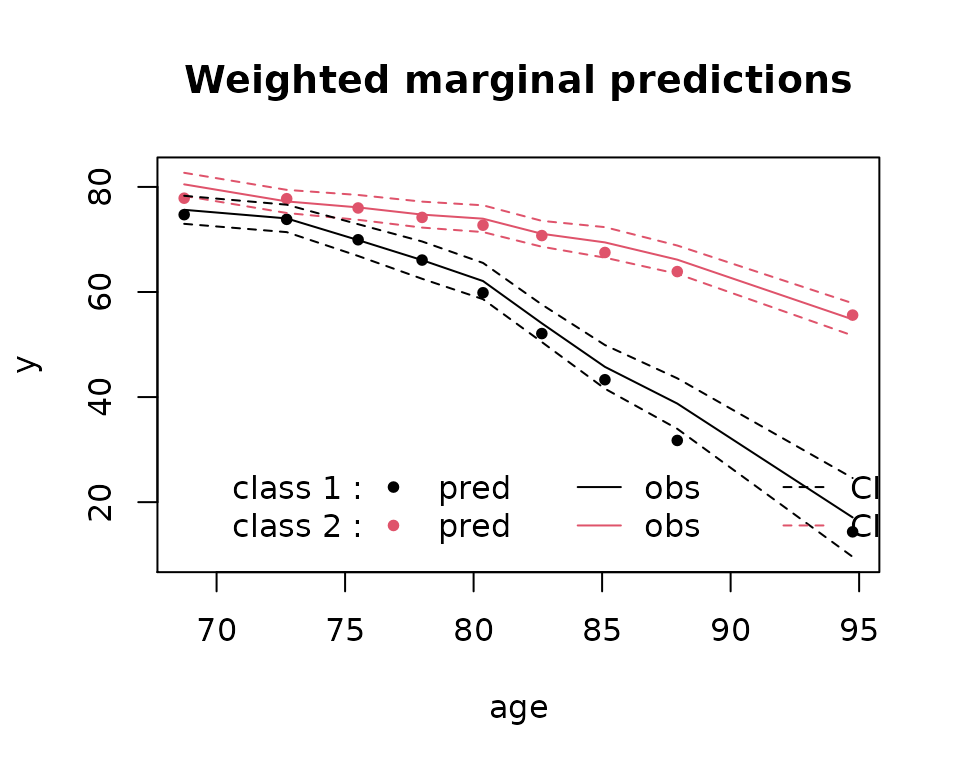
# fit of the longitudinal model: subject-specific predictions
plot(mj2,which="fit",var.time="age",marg=FALSE)
And the predictions of the model:
# plot of the baseline risk functions and survival functions
plot(mj2,which="baselinerisk",var.time="age")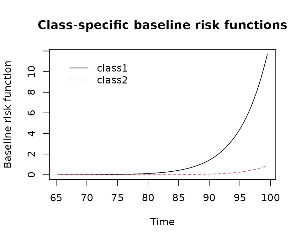
plot(mj2,which="survival",var.time="age")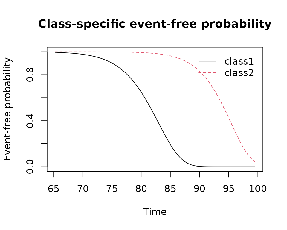
The model obtained with the first call of jointlcmm is not necessarily the maximum likelihood estimator for 2 classes. The model must be refitted with other initial values. There are different possibilities in the package:
random departure from the asymptotic distribution of the estimates under G=1
initial values chosen by the user
a grid search with replicates R times the random departures with a maximu of M iterations of the algorithm each time. The program finishes the estimation with the departure which gave the best log likelihood after the M iterations. This is what is recommended with latent class models to ensure the convergence toward the global maximum.
The grid search can take a lot of time as replicating R model estimation. I recommend to use 100 random departures and if possible between 30-50 iterations. Here, we will illustrate the procedure with less replicates and iterations to reduce the processing time.
# model with 2 latent classes and class-specific risk functions.
# multiple departures using a grid search
# (here, only a small gridsearch with 15 replicates and 10 iterations
# we recommend more replicated -50 to 100- and 30 iterations)
# Be careful, this might take a lot of time !!
mj2b <- gridsearch(rep = 15, maxiter = 10, minit = mj1, Jointlcmm(normMMSE ~ age65 +
        I(age65^2) + CEP, mixture =~ age65 + I(age65^2), random =~ age65 + I(age65^2),
        survival = Surv(age_init, agedem, dem) ~ CEP + male, hazard = "Weibull",
        subject = 'ID', data = paquidS, ng=2,verbose=F))
#> Warning in Surv(time = c(67.4167, 65.9167, 65.9167, 65.9167, 65.9167, 65.9167,
#> : type= 'mstate' is deprecated, use a factor variable as status
#> Warning in Surv(time = c(67.4167, 65.9167, 65.9167, 65.9167, 65.9167, 65.9167,
#> : type= 'mstate' is deprecated, use a factor variable as status
#> Warning in Surv(time = c(67.4167, 65.9167, 65.9167, 65.9167, 65.9167, 65.9167,
#> : type= 'mstate' is deprecated, use a factor variable as status
#> Warning in Surv(time = c(67.4167, 65.9167, 65.9167, 65.9167, 65.9167, 65.9167,
#> : type= 'mstate' is deprecated, use a factor variable as status
#> Warning in Surv(time = c(67.4167, 65.9167, 65.9167, 65.9167, 65.9167, 65.9167,
#> : type= 'mstate' is deprecated, use a factor variable as status
#> Warning in Surv(time = c(67.4167, 65.9167, 65.9167, 65.9167, 65.9167, 65.9167,
#> : type= 'mstate' is deprecated, use a factor variable as status
#> Warning in Surv(time = c(67.4167, 65.9167, 65.9167, 65.9167, 65.9167, 65.9167,
#> : type= 'mstate' is deprecated, use a factor variable as status
#> Warning in Surv(time = c(67.4167, 65.9167, 65.9167, 65.9167, 65.9167, 65.9167,
#> : type= 'mstate' is deprecated, use a factor variable as status
#> Warning in Surv(time = c(67.4167, 65.9167, 65.9167, 65.9167, 65.9167, 65.9167,
#> : type= 'mstate' is deprecated, use a factor variable as status
#> Warning in Surv(time = c(67.4167, 65.9167, 65.9167, 65.9167, 65.9167, 65.9167,
#> : type= 'mstate' is deprecated, use a factor variable as status
#> Warning in Surv(time = c(67.4167, 65.9167, 65.9167, 65.9167, 65.9167, 65.9167,
#> : type= 'mstate' is deprecated, use a factor variable as status
#> Warning in Surv(time = c(67.4167, 65.9167, 65.9167, 65.9167, 65.9167, 65.9167,
#> : type= 'mstate' is deprecated, use a factor variable as status
#> Warning in Surv(time = c(67.4167, 65.9167, 65.9167, 65.9167, 65.9167, 65.9167,
#> : type= 'mstate' is deprecated, use a factor variable as status
#> Warning in Surv(time = c(67.4167, 65.9167, 65.9167, 65.9167, 65.9167, 65.9167,
#> : type= 'mstate' is deprecated, use a factor variable as status
#> Warning in Surv(time = c(67.4167, 65.9167, 65.9167, 65.9167, 65.9167, 65.9167,
#> : type= 'mstate' is deprecated, use a factor variable as status
#> Warning in Surv(time = c(67.4167, 65.9167, 65.9167, 65.9167, 65.9167, 65.9167,
#> : type= 'mstate' is deprecated, use a factor variable as status

# An alternative is to directly choose the initial values and explore different
# plausible departures.
# The order of the B vector is the same as in the summary.
# Below, I keep the variance covariance parameters as in G=1. The other parameters are
# chosen according to values obtained above.
binit <- c(0,0.10,5,0.11,5.1,0,0,70,60,3,8,0,-5,13,mj1$best[9:15])
mj2c <- Jointlcmm(normMMSE ~ age65 + I(age65^2) + CEP, mixture =~ age65 + I(age65^2),
                  random =~ age65 + I(age65^2), survival = Surv(age_init, agedem, dem)
                  ~ CEP + male, hazard = "Weibull", subject = 'ID', data = paquidS,
                  ng=2,B=binit, verbose=FALSE)
#> Warning in Surv(time = c(67.4167, 65.9167, 65.9167, 65.9167, 65.9167, 65.9167,
#> : type= 'mstate' is deprecated, use a factor variable as status
# We can also start with a random departure:
mj2d <- Jointlcmm(normMMSE ~ age65 + I(age65^2) + CEP, mixture =~ age65 + I(age65^2),
                  random =~ age65 + I(age65^2), survival = Surv(age_init, agedem, dem)
                  ~ CEP + male, hazard = "Weibull", subject = 'ID', data = paquidS,
                  ng=2,B=random(mj1), verbose=FALSE)
#> Warning in Surv(time = c(67.4167, 65.9167, 65.9167, 65.9167, 65.9167, 65.9167,
#> : type= 'mstate' is deprecated, use a factor variable as status
In this example, we always converge to the same maximum whatever the departure but the latent classes might be exchanged.
# Comparison of the model estimations
summarytable(mj2,mj2b,mj2c,mj2d)
#>      G    loglik npm      BIC  %class1  %class2
#> mj2  2 -9337.187  21 18804.84 21.04208 78.95792
#> mj2b 2 -9337.187  21 18804.84 21.04208 78.95792
#> mj2c 2 -9337.187  21 18804.84 78.95792 21.04208
#> mj2d 2 -9337.187  21 18804.84 78.95792 21.04208
3.2 Model with more than 2 latent classes
Estimation of the models with 3 and 4 classes from default values (based on G=1 model estimates).
mj3 <- Jointlcmm(normMMSE ~ age65 + I(age65^2) + CEP, mixture =~ age65 + I(age65^2),
                 random =~ age65 + I(age65^2), survival = Surv(age_init, agedem, dem)
                 ~ CEP + male, hazard = "Weibull", subject = 'ID', data = paquidS,
                 ng = 3, B = mj1, verbose=FALSE)
#> Warning in Surv(time = c(67.4167, 65.9167, 65.9167, 65.9167, 65.9167, 65.9167,
#> : type= 'mstate' is deprecated, use a factor variable as status
#> Infinite parameters...
#> Last step values :
#>       b : -0.01460773 0.03389712 0.147233 3.443815 0.1038941 3.627087 0.1407469 3.791207 -0.2484353 -0.2007211 -0.00027607 64.64416 129.2885 3.296557 5.598101 7.900657 -6.886761 -6.096577 -5.304489 13.65079 14.58773 -14.83557 15.37587 3.81936 -5.796415 -3.343778 10.07244
#>       objective function : -9449.079
#>       Convergence criteria: parameters stability= 0
#>                           : function stability= 0
#>                           : best relative distance to maximum obtained (RDM)= 1

mj4 <- Jointlcmm(normMMSE ~ age65 + I(age65^2) + CEP, mixture =~ age65 + I(age65^2),
                 random =~ age65 + I(age65^2), survival = Surv(age_init, agedem, dem)
                 ~ CEP + male, hazard = "Weibull", subject = 'ID', data = paquidS,
                 ng = 4, B = mj1,verbose=F)
#> Warning in Surv(time = c(67.4167, 65.9167, 65.9167, 65.9167, 65.9167, 65.9167,
#> : type= 'mstate' is deprecated, use a factor variable as status
The program did not converge properly after 100 iterations (the maximum number of iterations specified by default). This is explained by the fact that the program converged to an non optimal point (local maximum). Indeed, when looking at the results (loglikelihood and estimates), the model mj3 converged toward the 1 class model and the model mj4 converged toward the 2 class model.
summarytable(mj1,mj2,mj3,mj4)
#>     G        loglik npm          BIC   %class1  %class2  %class3 %class4
#> mj1 1 -9.449079e+03  15 1.899135e+04 100.00000
#> mj2 2 -9.337187e+03  21 1.880484e+04  21.04208 78.95792
#> mj3 3 -1.000000e+09  27 2.000000e+09   0.00000  0.00000  0.00000
#> mj4 4 -9.337187e+03  33 1.887939e+04   0.00000 78.95792 21.04208       0
Such a problem may happen and the user should be careful with this issue. We can use other initial values to search for the global maximum in another part of the parameter space:
# For 3 classes, we need 6 additional parameters compared to the 2 class model:
# 1 proba + 2 Weibull + 3 polynomial parameters.

Binit <- rep(0, length(mj2$best) + 6)
Binit[c(2, 5:10, 12, 13, 15, 16, 18, 19:(length(Binit)))] <- mj2$best
Binit[c(1, 3, 4, 11, 14, 17)] <- c(0, 0.11, 4, 70, 0, 0)
mj3b <- Jointlcmm(normMMSE ~ age65 + I(age65^2) + CEP, mixture =~ age65 + I(age65^2),
                  random =~ age65 + I(age65^2), survival = Surv(age_init, agedem, dem)
                  ~ CEP + male, hazard = "Weibull", subject = 'ID', data = paquidS,
                  ng = 3, B = Binit, verbose=FALSE)

# For the 4 class model, we can start from the three class model:
Binit <- rep(0, length(mj3b$best) + 2 + 3 + 1)
Binit[c(1, 2, 4:7, 10:15, 17:19, 21:23, 25:length(Binit))] <- mj3b$best
Binit[c(3, 8, 9, 16, 20, 24)] <- c(-1, 0.1, 10, 60, 5, -10)
mj4b <- Jointlcmm(normMMSE ~ age65 + I(age65^2) + CEP, mixture =~ age65 + I(age65^2),
                  random =~ age65 + I(age65^2), survival = Surv(age_init, agedem, dem)
                  ~ CEP + male, hazard = "Weibull", subject = 'ID', data = paquidS,
                  ng = 4, B = Binit, verbose=FALSE)

# The best way is to use the grid search (although for the class, we consider only
# 10 replicates and 15 iterations at max so that it is not too long)
# But it is always better to try more random departures and iterations.
# 3 class model with gridsearch
mj3c <- gridsearch(rep = 10, maxiter = 15, minit = mj1, Jointlcmm(normMMSE ~ age65 +
                  I(age65^2) + CEP, mixture =~ age65 + I(age65^2), random =~ age65 +
                    I(age65^2), survival = Surv(age_init, agedem, dem) ~ CEP + male,
                   hazard = "Weibull", subject = 'ID', data = paquidS, ng =3, verbose=FALSE))

# 4 class model with gridsearch
mj4c <- gridsearch(rep = 10, maxiter = 15, minit = mj1, Jointlcmm(normMMSE ~ age65 +
                  I(age65^2) + CEP, mixture =~ age65 + I(age65^2), random =~ age65 +
                    I(age65^2), survival = Surv(age_init, agedem, dem) ~ CEP + male,
                  hazard = "Weibull", subject = 'ID', data = paquidS, ng = 4,verbose=F))
From the summary, we choose the 4 class model.
# summarytable by default
summarytable(mj1,mj2,mj3,mj3b,mj3c,mj4,mj4b,mj4c)
#>      G        loglik npm          BIC   %class1   %class2  %class3  %class4
#> mj1  1 -9.449079e+03  15 1.899135e+04 100.00000
#> mj2  2 -9.337187e+03  21 1.880484e+04  21.04208 78.957916
#> mj3  3 -1.000000e+09  27 2.000000e+09   0.00000  0.000000  0.00000
#> mj3b 3 -9.294952e+03  27 1.875764e+04  68.33667 13.026052 18.63727
#> mj3c 3 -9.294952e+03  27 1.875764e+04  18.63727 68.336673 13.02605
#> mj4  4 -9.337187e+03  33 1.887939e+04   0.00000 78.957916 21.04208  0.00000
#> mj4b 4 -9.267481e+03  33 1.873998e+04  69.13828  3.006012 14.02806 13.82766
#> mj4c 4 -9.279455e+03  33 1.876393e+04  14.22846  9.819639 48.89780 27.05411
# summary table with other measures for those who converged:
summarytable(mj1,mj2,mj3c,mj4b,which=c("npm","conv","loglik","BIC","SABIC","entropy","scoretest"))
#>      npm conv    loglik      BIC    SABIC   entropy scoretest
#> mj1   15    1 -9449.079 18991.35 18943.74 1.0000000         0
#> mj2   21    1 -9337.187 18804.84 18738.18 0.5905253         0
#> mj3c  27    1 -9294.952 18757.64 18671.94 0.5419923         0
#> mj4b  33    1 -9267.481 18739.98 18635.24 0.6052817         0
# plots
summaryplot(mj1,mj2,mj3c,mj4b,which=c("BIC","entropy"))
# score test statistics for the independence assumption
ST <- c(mj1$scoretest[1],mj2$scoretest[1],mj3c$scoretest[1],mj4b$scoretest[1])
plot(ST ~ c(1:4),type="l",bty='n',main="Score test", xlab="number of classes", ylab="")
The score test statistics rejects the conditional independence at the 5% level but the shape of the curve of ST according to the number of class (with the asymptot) tells us that we will probably never reach the significance level.
4.1. Summary of the estimation
The summary gives all the important information
summary(mj4b)
#> Joint latent class model for quantitative outcome and competing risks
#>      fitted by maximum likelihood method
#>
#> Jointlcmm(fixed = normMMSE ~ age65 + I(age65^2) + CEP, mixture = ~age65 +
#>     I(age65^2), random = ~age65 + I(age65^2), subject = "ID",
#>     ng = 4, survival = Surv(age_init, agedem, dem) ~ CEP + male,
#>     hazard = "Weibull", data = paquidS)
#>
#> Statistical Model:
#>      Dataset: paquidS
#>      Number of subjects: 499
#>      Number of observations: 2213
#>      Number of latent classes: 4
#>      Number of parameters: 33
#>      Event 1:
#>         Number of events: 128
#>         Class-specific hazards and
#>         Weibull baseline risk function
#>
#> Iteration process:
#>      Convergence criteria satisfied
#>      Number of iterations:  37
#>      Convergence criteria: parameters= 5.1e-07
#>                          : likelihood= 1.9e-09
#>                          : second derivatives= 2e-11
#>
#> Goodness-of-fit statistics:
#>      maximum log-likelihood: -9267.48
#>      AIC: 18600.96
#>      BIC: 18739.98
#>      Score test statistic for CI assumption: 30.667 (p-value=0)
#>
#> Maximum Likelihood Estimates:
#>
#> Fixed effects in the class-membership model:
#> (the class of reference is the last class)
#>
#>                        coef       Se     Wald p-value
#> intercept class1    0.65212  0.23030    2.832 0.00463
#> intercept class2   -1.43834  0.35000   -4.110 0.00004
#> intercept class3   -0.24518  0.24883   -0.985 0.32447
#>
#> Parameters in the proportional hazard model:
#>
#>                                        coef       Se     Wald p-value
#> event1 +/-sqrt(Weibull1) class 1    0.10121  0.00039  259.468 0.00000
#> event1 +/-sqrt(Weibull2) class 1    7.04817  0.82048    8.590 0.00000
#> event1 +/-sqrt(Weibull1) class 2    0.11421  0.00080  142.611 0.00000
#> event1 +/-sqrt(Weibull2) class 2    5.57068  0.73739    7.555 0.00000
#> event1 +/-sqrt(Weibull1) class 3    0.10955  0.00039  278.060 0.00000
#> event1 +/-sqrt(Weibull2) class 3    6.39438  0.42368   15.093 0.00000
#> event1 +/-sqrt(Weibull1) class 4    0.10567  0.00037  284.419 0.00000
#> event1 +/-sqrt(Weibull2) class 4    6.91442  0.50272   13.754 0.00000
#> CEP                                -0.66581  0.26347   -2.527 0.01150
#> male                                0.43642  0.29474    1.481 0.13869
#>
#> Fixed effects in the longitudinal model:
#>
#>                         coef       Se     Wald p-value
#> intercept class1    65.30224  3.38070   19.316 0.00000
#> intercept class2    83.22520  9.26192    8.986 0.00000
#> intercept class3    65.50576  4.93596   13.271 0.00000
#> intercept class4    57.39464  5.26996   10.891 0.00000
#> age65 class1         4.62182  3.73925    1.236 0.21645
#> age65 class2       -64.10601 16.27520   -3.939 0.00008
#> age65 class3        15.15503  6.72450    2.254 0.02421
#> age65 class4        19.31410  6.06023    3.187 0.00144
#> I(age65^2) class1   -3.25830  1.08339   -3.008 0.00263
#> I(age65^2) class2   16.81961  6.30158    2.669 0.00761
#> I(age65^2) class3  -16.26249  2.15040   -7.563 0.00000
#> I(age65^2) class4  -11.44706  1.80170   -6.353 0.00000
#> CEP                 12.80547  1.20940   10.588 0.00000
#>
#>
#> Variance-covariance matrix of the random-effects:
#>             intercept     age65 I(age65^2)
#> intercept   235.93031
#> age65      -251.67607  439.6307
#> I(age65^2)   74.24157 -139.0736   45.49113
#>
#>                               coef       Se
#> Residual standard error    9.94241  0.19331
4.2. Evaluation of the classification
A major element of joint latent class models is the posterior classification, and the discriminatory power of this classification.
# table with the posterior classification
head(mj4b$pprob)
#>   ID class     probYT1      probYT2      probYT3   probYT4
#> 1  1     1 0.458599701 7.289192e-02 1.526894e-01 0.3158190
#> 2  2     4 0.002627611 1.713013e-06 4.695802e-01 0.5277904
#> 3  3     1 0.432859275 7.912249e-02 2.306033e-01 0.2574149
#> 4  4     4 0.260838221 2.008358e-15 9.800983e-03 0.7293608
#> 5  5     1 0.608782214 4.225492e-21 2.848206e-05 0.3911893
#> 6  6     4 0.009333558 2.860090e-14 1.728421e-02 0.9733822
# output for classification evaluation
postprob(mj4b)
#>
#> Posterior classification based on longitudinal and time-to-event data:
#>   class1 class2 class3 class4
#> N 345.00  15.00  70.00  69.00
#> %  69.14   3.01  14.03  13.83
#>
#> Posterior classification table:
#>      --> mean of posterior probabilities in each class
#>         prob1  prob2  prob3  prob4
#> class1 0.7188 0.0093 0.0817 0.1902
#> class2 0.0355 0.8873 0.0518 0.0254
#> class3 0.0565 0.0319 0.7978 0.1137
#> class4 0.1155 0.0000 0.0621 0.8224
#>
#> Posterior probabilities above a threshold (%):
#>          class1 class2 class3 class4
#> prob>0.7  49.28  86.67  67.14  71.01
#> prob>0.8  40.87  86.67  54.29  65.22
#> prob>0.9  31.30  73.33  52.86  59.42
#>
#>
#> Posterior classification based only on longitudinal data:
#>   class1 class2 class3 class4
#> N 344.00  16.00  68.00  71.00
#> %  68.94   3.21  13.63  14.23
#>
4.3 Graphs for the fit
We can assess the fit of the model by comparing the predictions to the observations by time intervals.
# overall
plot(mj4b, which = "fit", var.time = "age65", marg = F, break.times = 10, bty = "l",
     ylab = "normMMSE", xlab = "Age in decades from 65 years",shades=TRUE)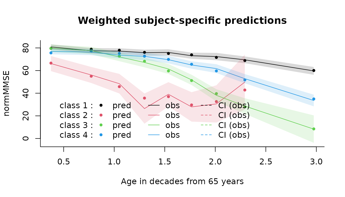
# by covariate profile
par(mfrow=c(1,2))
plot(mj4b, which = "fit", var.time = "age65", marg = F, break.times = 10, bty = "l",
     ylab = "normMMSE", xlab = "Age in decades from 65 years",subset = dem == 1,
     main="diagnosed as demented",shades=TRUE)
plot(mj4b, which = "fit", var.time = "age65", marg = F, break.times = 10, bty = "l",
     ylab = "normMMSE", xlab = "Age in decades from 65 years",subset = dem == 0,
     main="non diagnosed as demented",shades=TRUE)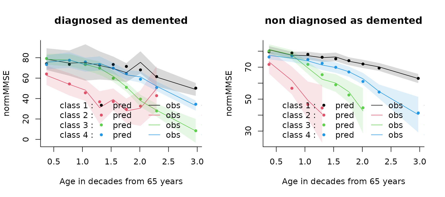
The residuals of the longitudinal part:
plot(mj4b)4.4. Graph of predicted trajectories according to a profile of covariates
datnew <- data.frame(age65 = seq(0, 3, length=100))
datnew$male <- 0
datnew$CEP <- 0
# computation of the predictions
mj4b.pred <- predictY(mj4b, newdata = datnew, var.time = "age65")
plot(mj4b.pred, bty = "l", ylim = c(0, 80), legend.loc = "bottomleft",
     ylab = "normMMSE", xlab = "age in decades from 65 years", lwd = 2)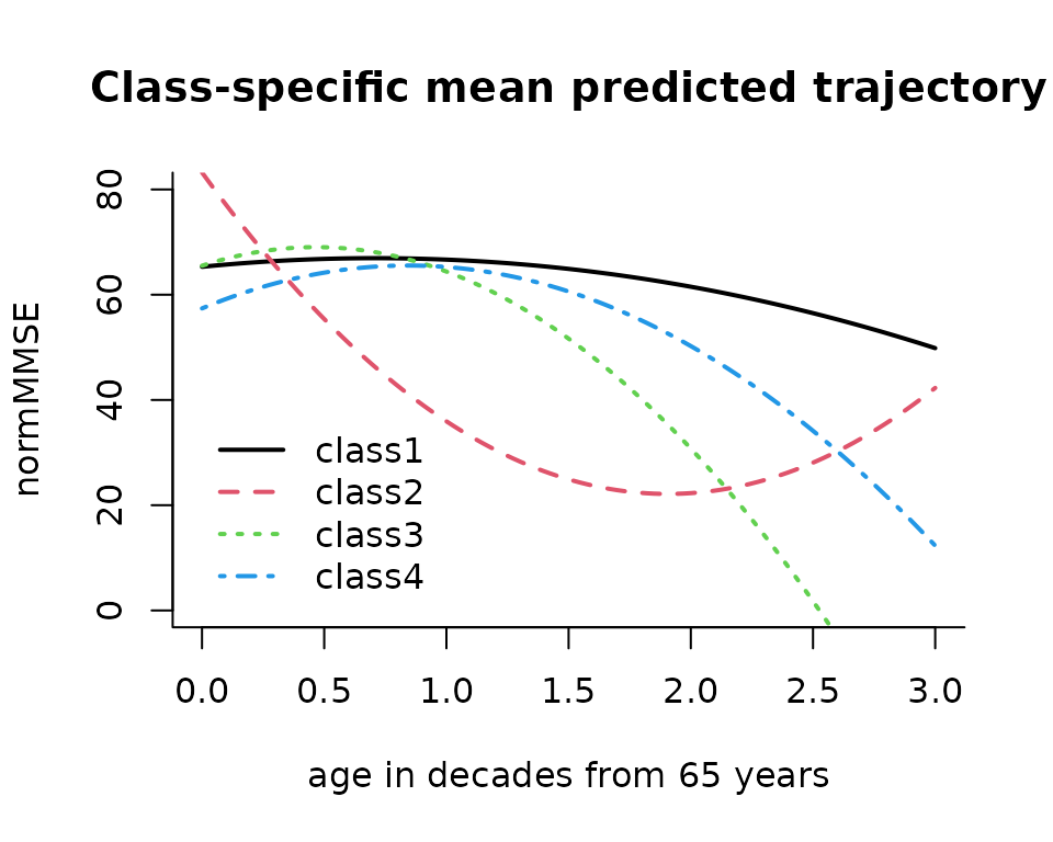
4.5. Graph of predicted cumulative incidence according to a profile of covariates
# graph of predicted survival trajectory for the reference group
plot(mj4b, which = "survival", lwd = 2, legend.loc = F, bty = "l",
     xlab = "age in years", ylab = "dementia-free probability")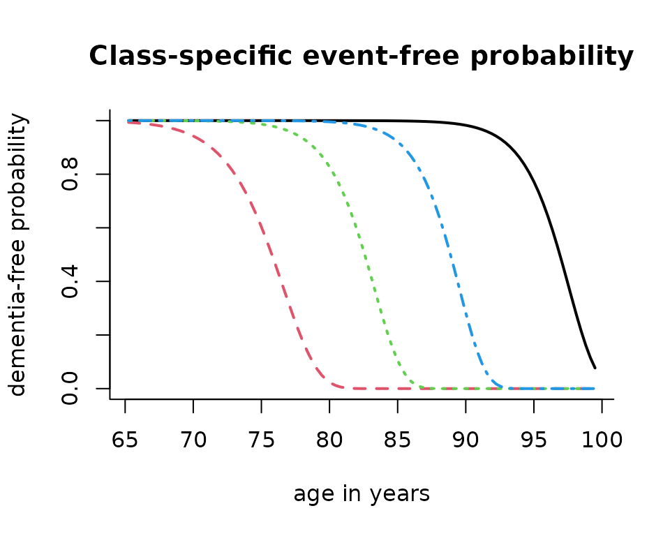
# computation of the cumulative incidence for a specific profile of covariates
cuminc0 <- cuminc(mj4b,time = seq(65,95,by=1))
cuminc1 <- cuminc(mj4b,time = seq(65,95,by=1),CEP=1,male=1)
# plot of cumulative incidences
par(mfrow=c(1,2))
plot(cuminc0,title="CEP=0 and male=0")
plot(cuminc1,lty=2,title="CEP=1 and male=1")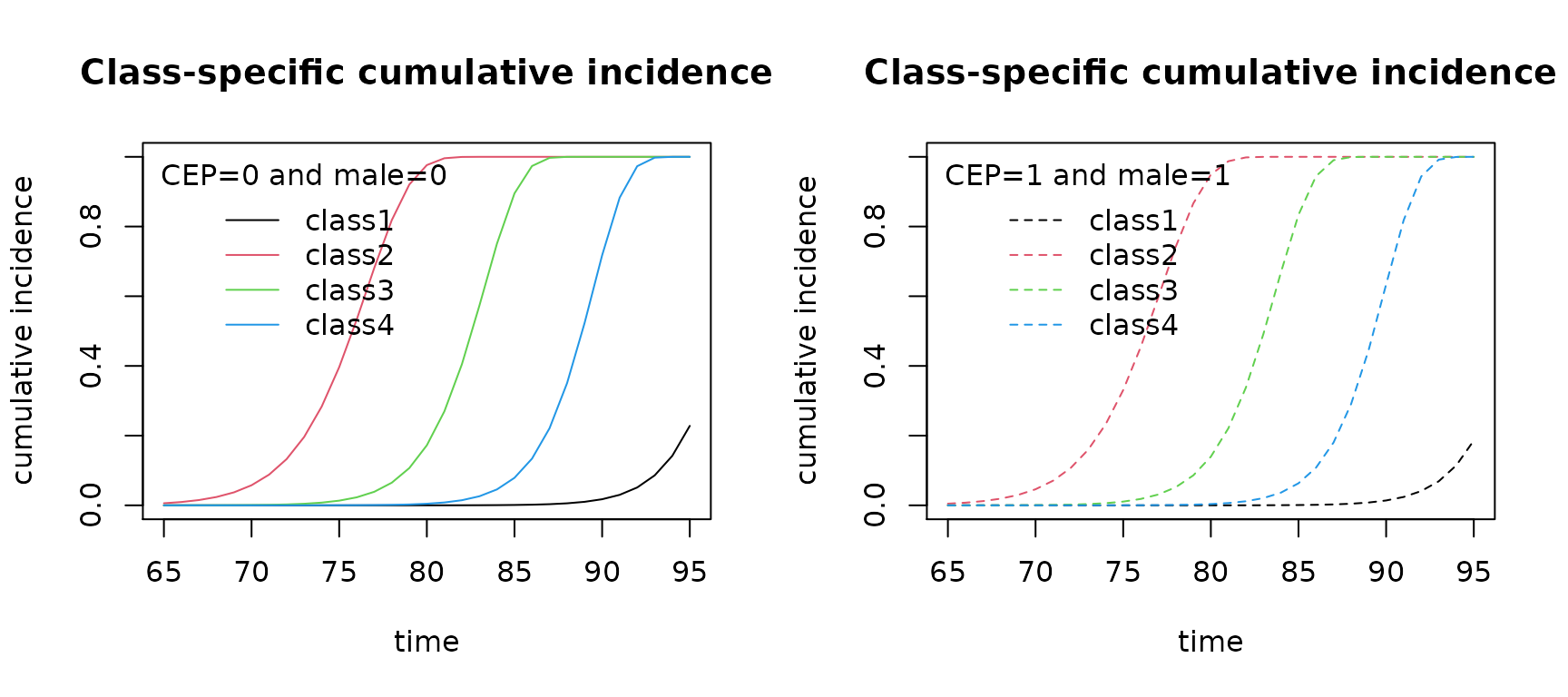
C. To go further …
1. Individual dynamic prediction
The joint latent class model can be used to provide individual dynamic prediction of the event from the observed repeated measures of the marker. This is usually done for a “new” subject (not in the estimation data) but for the class, we focus on subject 72:
paq72 <- paquidS[which(paquidS$ID == 72), ]
# prediction computation
dynp <- dynpred(mj4b, paq72, landmark = c(80, 90), var.time = "age65",
                horizon = c(1, 3, 5, 8, 9), fun.time = function(x) { 10 * x + 65 },
                draws = TRUE)
#>       ID landmark horizon    pred_50   pred_2.5  pred_97.5
#>  [1,] 72       80       1 0.01792567 0.01025557 0.02845754
#>  [2,] 72       80       3 0.07781886 0.04932919 0.11742875
#>  [3,] 72       80       5 0.17582383 0.12074292 0.24851275
#>  [4,] 72       80       8 0.30572794 0.22399247 0.40675696
#>  [5,] 72       80       9 0.34106835 0.25532066 0.43885727
#>  [6,] 72       90       1 0.08007715 0.03678548 0.15947501
#>  [7,] 72       90       3 0.22151193 0.10915870 0.42406186
#>  [8,] 72       90       5 0.31316574 0.18850276 0.53375716
#>  [9,] 72       90       8 0.58655983 0.39958818 0.81559952
#> [10,] 72       90       9 0.72133824 0.50421389 0.94933195
# graph of predictions
plot(dynp, landmark = 80, ylim = c(55, 85, 0, 1), col = c(1,2), pch = 20,
     ylab = "normMMSE", main = "At landmark age 80", xlab = "age in years")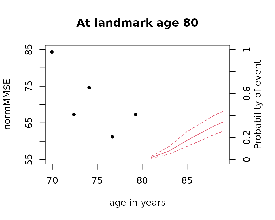
plot(dynp, landmark = 90, ylim = c(55, 85, 0, 1), col = c(1,2), pch = 20,
     ylab = "normMMSE", main = "At landmark age 90", xlab = "age in years")
When the objective is to provide dynamic predictions, the predictive power of the model should be specifically checked using appropriate techniques. The package has an internal measure, the EPOCE which quantifies the pronostic information. For measures such as the AUC or Brier Score, other packages can be used from the dynamic predictions obtained with Jointlcmm, for instance timeROC (Blanche et al., Biometrics 2015).
Here is an example of the use of EPOCE:
# definition of the prediction times
landmark <- c(70, 72, 75, 77, 80, 82, 85, 87, 90)
# calculation of the measure for each model. Be careful with the function which links
# the time in the longitudinal model and the time in the survival model (fun.time)
epoce1 <- epoce(mj1, pred.times = landmark, var.time = "age65",fun.time =
                  function(x) { 10 * x + 65 })
#> Warning in Surv(time = c(67.4167, 65.9167, 65.9167, 65.9167, 65.9167, 65.9167,
#> : type= 'mstate' is deprecated, use a factor variable as status
#> Be patient, epoce function is running ...
#> The program took 0.32 seconds
epoce2 <- epoce(mj2, pred.times = landmark, var.time = "age65",fun.time =
                  function(x) { 10 * x + 65 })
#> Warning in Surv(time = c(67.4167, 65.9167, 65.9167, 65.9167, 65.9167, 65.9167,
#> : type= 'mstate' is deprecated, use a factor variable as status
#> Be patient, epoce function is running ...
#> The program took 0.58 seconds
epoce3 <- epoce(mj3b, pred.times = landmark, var.time = "age65",fun.time =
                  function(x) { 10 * x + 65 })
#> Warning in Surv(time = c(67.4167, 65.9167, 65.9167, 65.9167, 65.9167, 65.9167,
#> : type= 'mstate' is deprecated, use a factor variable as status
#> Be patient, epoce function is running ...
#> The program took 0.86 seconds
epoce4 <- epoce(mj4b, pred.times = landmark, var.time = "age65",fun.time =
                  function(x) { 10 * x + 65})
#> Warning in Surv(time = c(67.4167, 65.9167, 65.9167, 65.9167, 65.9167, 65.9167,
#> : type= 'mstate' is deprecated, use a factor variable as status
#> Be patient, epoce function is running ...
#> The program took 1.2 seconds
# computation of the differences in EPOCE
diff23 <- Diffepoce(epoce2, epoce3)
diff34 <- Diffepoce(epoce3, epoce4)
# and the graphs for the results
par(mfrow = c(1, 2))
plot(epoce1, ylim = c(0.5, 1.5), main = "cross-validated EPOCE estimates",bty = "l")
plot(epoce2, add = TRUE, col = 2, lty = 2)
plot(epoce3, add = TRUE, col = 3, lty = 3)
plot(epoce4, add = TRUE, col = 4, lty = 4)
legend("topright", legend = c("G=1", "G=2", "G=3", "G=4"), col = 1:4,lty = 1:4,
       bty = "n")
plot(diff23, main = "Difference in EPOCE estimates", lty = c(1, 2, 2),pch = 20,
     ylim = c(-0.05, 0.30), bty = "l")
plot(diff34, add = T, main = "Difference in EPOCE estimates", col = 4,
     lty = c(1, 2, 2), pch = 18)
legend("topleft", legend = c("G=2/G=3", "G=3/G=4", "95%TI", "95%TI"),
       ncol = 2, col = c(1, 4, 1, 4), lty = c(1, 1, 2, 2), pch = c(20, 18, 20, 18),
       bty = "n")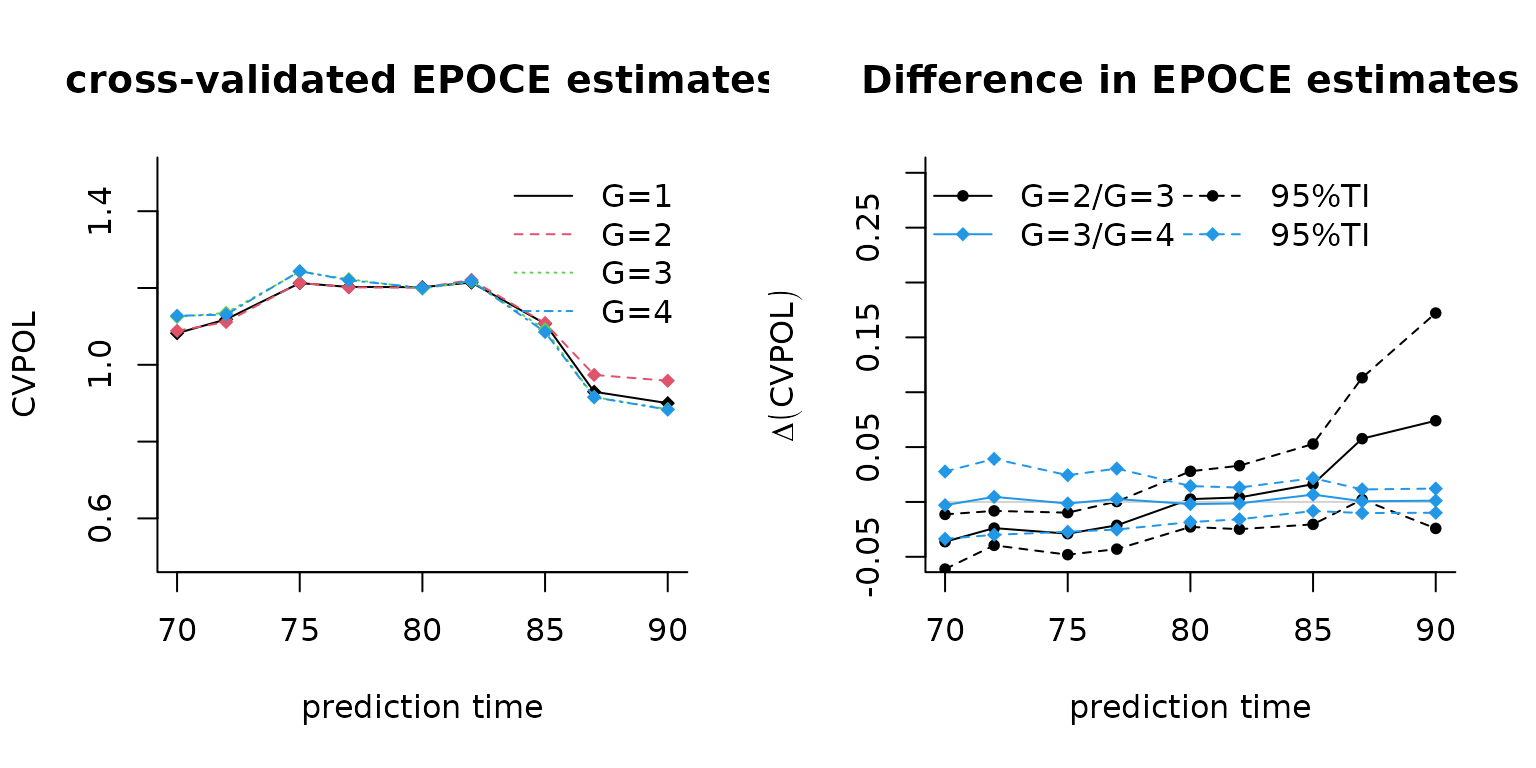
Here the model with 3 latent classes seems to have a better predictive power than the 4 class model.
2. Competing risks
Jointlcmm function can account for competing risks with the same structure of call. The only difference is in the definition of the time to event which is the minimum time between all the causes of event and the censoring. The indicator of event also indicates 0 for censoring or k for cause k. Suppose we have further information in the paquidS sample, namely a variable Age_CR that includes the first event between dementia and death, and Indic_CR that indicates the cause of event, dementia or death before dementia. In the following we give some examples of joint latent class models with competing risks.
# model with G=1 with Weibull for both events
mj1_CR <- Jointlcmm(normMMSE ~ age65+I(age65^2) + CEP, random =~  age65+I(age65^2),
                         survival = Surv(age_init, Age_CR, Indic_CR) ~ CEP + male,
                         hazard = "Weibull", subject = 'ID', data = paquidS_CR, ng = 1)
In the regression, we can consider specific effects with cause() :
# model with G=1 and cause-specific effects of CEP and male
mj1_CR_CS <- Jointlcmm(normMMSE ~ age65+I(age65^2) + CEP, random =~ age65+I(age65^2),
                 survival = Surv(age_init, Age_CR, Indic_CR)  ~ cause(CEP)
                + cause(male), hazard = "Weibull", subject = 'ID', data = paquidS_CR,
                ng = 1,verbose=F)
Note that different baseline risk functions can be considered for the two events:
mj1_CR_WS <- Jointlcmm(normMMSE ~ age65+I(age65^2) + CEP, random =~  age65+I(age65^2),
                         survival = Surv(age_init, Age_CR, Indic_CR) ~ CEP + male,
                         hazard = c("Weibull","splines"), subject = 'ID', data = paquidS_CR, ng = 1)
summary(mj1_CR_WS)
We can now use the same technique of estimation with G>1 for this model with competing risks …