Predicted cumulative incidence of event according to a profile of covariates

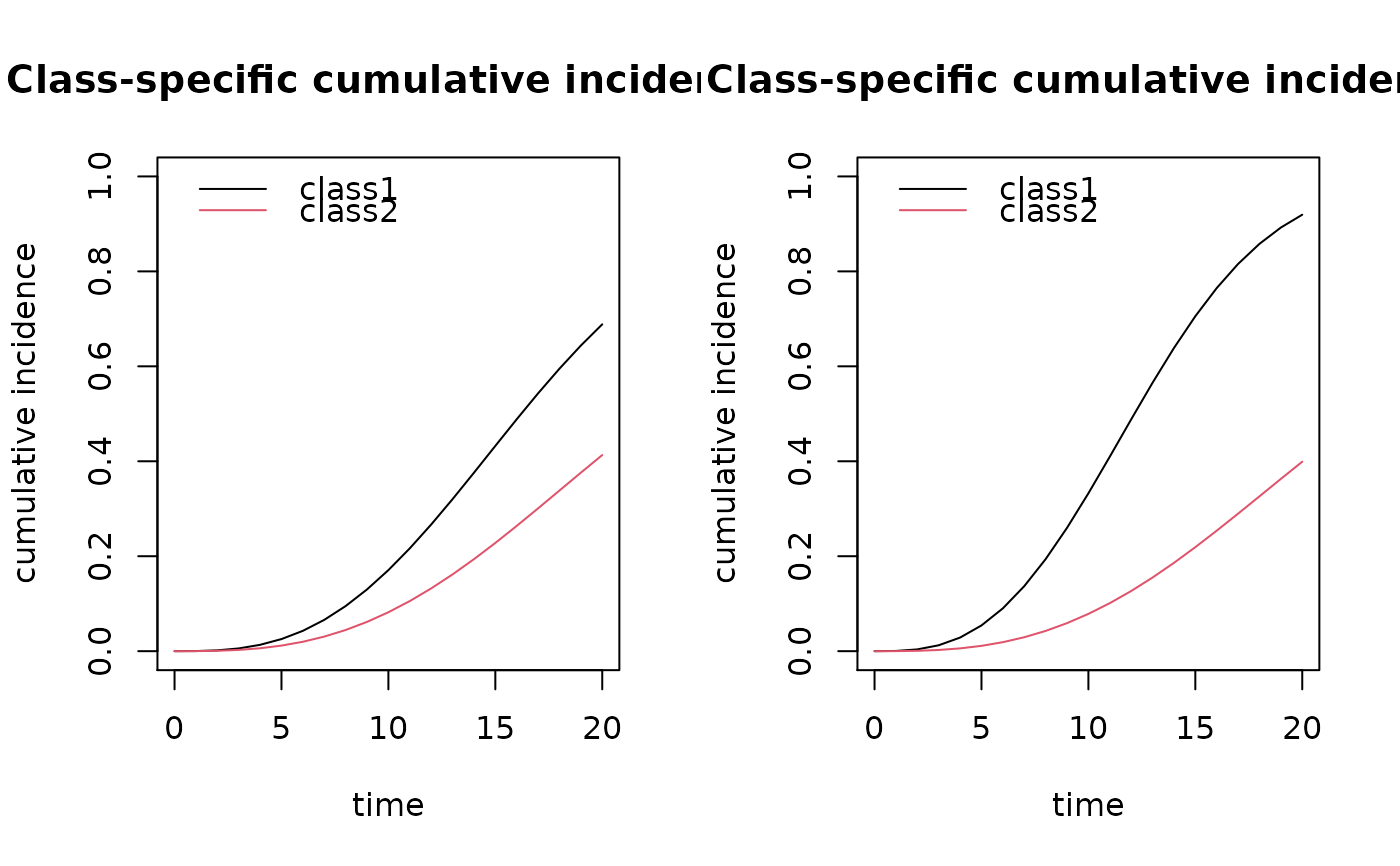
This function computes the predicted cumulative incidence of each cause of event according to a profile of covariates from a joint latent class model. Confidence bands can be computed by a Monte-Carlo method.

Usage

cuminc(x, time, draws = FALSE, ndraws = 2000, integrateOptions = NULL, ...)

Arguments

x: an object inheriting from class Jointlcmm or mpjlcmm
time: a vector of times at which the cumulative incidence is calculated
draws: optional boolean specifying whether a Monte Carlo approximation of the posterior distribution of the cumulative incidence is computed and the median, 2.5% and 97.5% percentiles are given. Otherwise, the predicted cumulative incidence is computed at the point estimate. By default, draws=FALSE.
ndraws: if draws=TRUE, ndraws specifies the number of draws that should be generated to approximate the posterior distribution of the predicted cumulative incidence. By default, ndraws=2000.
integrateOptions: optional list specifying the subdivisions, rel.tol and stop.on.error options (see ?integrate).
...: further arguments, in particular values of the covariates specified in the survival part of the joint model.

Value

An object of class cuminc containing as many matrices as profiles defined by the covariates values. Each of these matrices contains the event-specific cumulative incidences in each latent class at the different times specified.

Author

Viviane Philipps and Cecile Proust-Lima

Examples

m2 <- Jointlcmm(fixed= Ydep1~Time*X1,mixture=~Time,random=~Time,
classmb=~X3,subject='ID',survival = Surv(Tevent,Event)~X1+mixture(X2),
hazard="3-quant-splines",hazardtype="PH",ng=2,data=data_lcmm,
B=c(0.64,-0.62,0,0,0.52,0.81,0.41,0.78,0.1,0.77,-0.05,10.43,11.3,-2.6,
-0.52,1.41,-0.05,0.91,0.05,0.21,1.5))

par(mfrow=c(1,2))
plot(cuminc(m2,time=seq(0,20),X1=0,X2=0), ylim=c(0,1))
plot(cuminc(m2,time=seq(0,20),X1=0,X2=1), ylim=c(0,1))