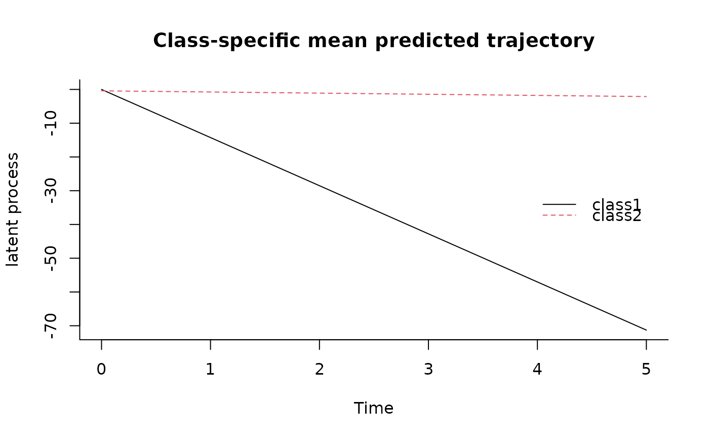
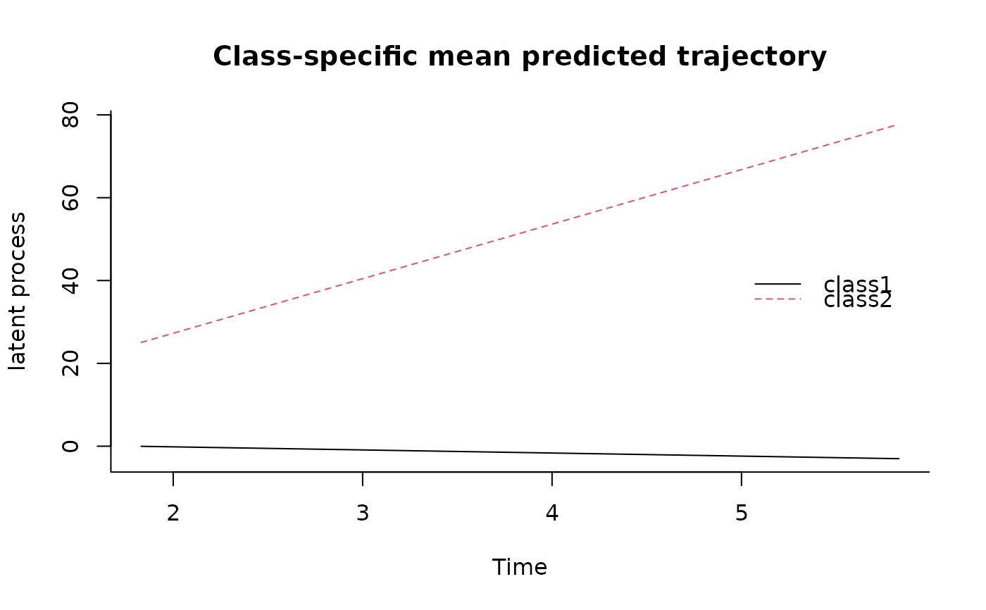
Plot of predicted trajectories and link functions

This function provides the class-specific predicted trajectories stemmed from a hlme, lcmm, multlcmm or Jointlcmm object.

Usage

# S3 method for predictL
plot(x, legend.loc = "topright", legend, add = FALSE, shades = FALSE, ...)

# S3 method for predictY
plot(
  x,
  outcome = 1,
  legend.loc = "topright",
  legend,
  add = FALSE,
  shades = FALSE,
  ...
)

# S3 method for predictYcond
plot(x, legend.loc = "topleft", legend, add = FALSE, shades = TRUE, ...)

Arguments

x

an object inheriting from classes predictL, predictY or predictlink representing respectively the predicted marginal mean trajectory of the latent process, the predicted marginal mean trajectory of the longitudinal outcome, or the predicted link function of a fitted latent class model.

legend.loc

keyword for the position of the legend from the list "bottomright", "bottom", "bottomleft", "left", "topleft","top", "topright", "right" and "center".

legend

character or expression to appear in the legend. If no legend should be added, "legend" should be NULL.

add

logical indicating if the curves should be added to an existing plot. Default to FALSE.

shades

logical indicating if confidence intervals should be represented with shades. Default to FALSE, the confidence intervals are represented with dotted lines.

...

other parameters to be passed through to plotting functions or to legend

outcome

for predictY and multivariate model fitted with multlcmm only, the outcome to consider.

See also

hlme, lcmm, Jointlcmm, multlcmm

Author

Cecile Proust-Lima, Benoit Liquet and Viviane Philipps

Examples

################# Prediction from linear latent class model
## fitted model
m<-lcmm(Y~Time*X1,mixture=~Time,random=~Time,classmb=~X2+X3,
subject='ID',ng=2,data=data_hlme,B=c(0.41,0.55,-0.18,-0.41,
-14.26,-0.34,1.33,13.51,24.65,2.98,1.18,26.26,0.97))
## newdata for predictions plot
newdata<-data.frame(Time=seq(0,5,length=100),
X1=rep(0,100),X2=rep(0,100),X3=rep(0,100))
plot(predictL(m,newdata,var.time="Time"),legend.loc="right",bty="l")

## data from the first subject for predictions plot
firstdata<-data_hlme[1:3,]
plot(predictL(m,firstdata,var.time="Time"),legend.loc="right",bty="l")


 # \dontrun{
################# Prediction from a joint latent class model
## fitted model - see help of Jointlcmm function for details on the model
m3 <- Jointlcmm(fixed= Ydep1~Time*X1,mixture=~Time,random=~Time,
classmb=~X3,subject='ID',survival = Surv(Tevent,Event)~X1+mixture(X2),
hazard="3-quant-splines",hazardtype="PH",ng=3,data=data_lcmm,
B=c(0.7576, 0.4095, -0.8232, -0.2737, 0, 0, 0, 0.2838, -0.6338, 
2.6324, 5.3963, -0.0273, 1.398, 0.8168, -15.041, 10.164, 10.2394, 
11.5109, -2.6219, -0.4553, -0.6055, 1.473, -0.0383, 0.8512, 0.0389, 
0.2624, 1.4982))
# class-specific predicted trajectories 
#(with characteristics of subject ID=193)
data <- data_lcmm[data_lcmm$ID==193,]
plot(predictY(m3,newdata=data,var.time="Time"),bty="l")

# }